15 Most Basic Things of Excel – Every Excel-user Must Know (Part – 1)

It is globally accepted that MS-Excel is the most preferred and premium tool for Data Analysis at low level and for most numerical and statistical operations. Due to its versatile ability, excel is the most popular and preferable tool among all spreadsheet software. But all excel users do not have the same level of proficiency. Some are novice and some familiar. Some features may be very tough or tricky for the novice, at least until they learn or are explained. There are some basics that one must know to use the Excel effectively and efficiently. You will be competent excel user by conquering these skills.

(1.) Work Area and Print Area

Each-n-every software has an area where you work, just like a stage where an actor performs his role. Here, we’ll talk about ‘work area’, which simply denotes an area which will let you put your work. Every excel file consists of a set of spreadsheets. Every spreadsheet is called ‘Worksheet’ or simply a ‘sheet’. An excel file is called ‘workbook’. Every workbook contains a worksheet or group of worksheets. Thus, ‘Worksheet’ is a work area of excel. A worksheet is a sheet with columns and rows. An intersection of a row and a column is known as a ‘cell’. There are thousands of cells spread on a sheet, that’s why it is called spreadsheet. While printing, by default the printer considers area from upper left cell to the bottom right used cell as print area. According to page size it splits data across pages. Print area can be defined by selecting desired area to be printed and just clicking a ‘Set Print Area’ button. Doing this, only defined area will get printed instead of the whole used area of the sheet.

(2.) Fill Handle

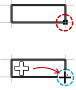
This is the most helpful and time saving smart tool. It is slight bigger square shape at bottom right corner of the cell cursor. It moves with the cell cursor. This tool helps to fill data series by dragging it across row or column. E.g. months from ‘Jan’ to ‘Dec’ or sequential numeric series like 1,2,3 ……n etc. Mouse pointer will get changed from big outlined plus sign to smaller and dark plus sign. This indicates that excel is now ready to fill series by dragging it across columns or rows. If two consecutive numbers are in ascending order then every next figure will get increased by the difference of those two numbers. Similarly, if they are in descending order then every next figure will get decreased by the difference of those two numbers. It also fills alpha-numeric series like a.1, a.2., a.3 … etc. Last character must be number to perform auto-increment of such numbers. Month names and week names (short and full both) also get filled automatically with the help of the fill-handle, because they are definite. Values defined in custom-list also get filled with the help of the fill handle. Double clicking on the fill-handle will fill values/formula downwards into the current column up to last used cell of left or right column. It looks into left column first, and then right, if the left column to the current column is empty. It will stop filling values if any of the cells of the active column contains any value. Thus, the fill-handle is very helpful for fast data-entry work which saves time and increases accuracy, avoiding errors/duplication.

(3.) Status Bar

‘Status’ bar simply displays various statuses. It displays average, count, max and sum of selected cells having numeric values. It also counts cells having text values. We need this type of figures very frequently. Perhaps this is the easiest and fastest technique/way to get sum, max, average and count of selected values quickly. Even novice can use this tip confidently. It gives handy options to switch between frequently used views like Normal, Page Layout and Page Break View. With Office 2007, users can easily zoom-in or zoom-out with zoom bar. Recording macro and stopping macro can also be managed from the status bar.

(4.) Interface Differences

There are vast interface differences between ribbon and non-ribbon versions. With office 2007 most of the features and options are available on ribbon, which were available on toolbars in previous versions. Menu names have been changed to ribbon titles and most of the commands have taken the form of icons and placed on big horizontal bar known as ‘Ribbon’. This main difference made office more attractive and popular. Due to this difference, earlier versions are known as non-ribbon versions and Office-2007 and higher versions are known as ribbon versions. Live preview is also one of the most significant improvements. Moreover, plenty of colors can now be used to decorate or highlight fonts, cells, borders, charts and drawing objects or shapes. Every user wants to use MS-Excel according to their styles and requirements. Use of various options may vary from user to user. To facilitate such facility, “Options” command is available in ‘Tools’ menu. In ribbon versions it is available in “Office Button” (in 2007) menu or “File” (in 2010 and higher) menu.

(5.) Formula Bar and Name box/Address box

This is the main part of any spreadsheet software. It is located just above the column titles of a worksheet. The formula bar has two parts. Left part is smaller and shows usually current cell address or cell address of the top-left cell of the selected cells. That’s why it is known as ‘Name Box’ or ‘Address Box’. It also shows selected number of rows and columns while selecting cells. Suppose there are 12 rows and 8 columns selected then it will indicate it as “12R x 8C” while selecting. As soon as the process of selecting cells gets completed, it will show cell address of the top-left cell. You can resize the Name-box. Right part is the actual ‘Formula bar’, which shows whatever is in the current cell. If the cell contains static text/value than it will show that content itself. If the cell contains formula and/or function then it will show that formula and/or function. The formula bar can be vertically resized if the formula is longer. In non-ribbon versions, it got resized automatically but with overlapping the column heading and few of the top visible rows. This limitation has been removed in ribbon versions. There is a toggle formula-bar resize button at right end of the formula-bar. By default, it resizes the formula-bar up to 3 lines. User can resize the bar even more. It also remembers the resized height of formula-bar. We listed the first five most basic things that every Excel user should know. To get more idea about the other basic things, continue reading 15 Most Basic Things of Excel (Part-2).